Math might not be everyone’s favorite subject, but Excel makes it a whole lot friendlier with its array of mathematical formulas. Let’s peek under the hood and understand some of the most commonly used ones.

But wait… What if I don’t want to know the total for all shoes sold? What if I only care about the red ones? And WHAT ABOUT THE FRUIT?!?! Maybe I only care about oranges? Well, there are options for that also, and I’ll be providing some of the most commonly used ones in this post below each of the ‘everything’ versions of the formulas.

Sorry not sorry; I’ve seen these crazy examples for years and I finally had a chance to make my own, so you can deal with it.

Me, the author<3

SUM()

Syntax: SUM(number1, [number2], …)

How I remember it: Sum(of everything in this range) or Sum(of these specific values)

This function is Excel’s basic arithmetic superstar. It adds up all the numbers in the specified range. If you need to find the total sales for a week or sum up expenses for a month, SUM is your go-to function.

Example: “=SUM(A1:A10)” adds up all the numbers from cells A1 to A10.

I’ll provide visual examples for this first one, so that you can see the structure as it appears in Excel, but they’re all pretty similar, so I don’t intend to do examples for each formula.

The picky one: SUMIFS()

Syntax: SUMIFS(sum_range, criteria_range1, criteria1, [criteria_range2, criteria2], …)

How I remember it: Sumifs(All values in this range,When the value in this other range, equals THIS)

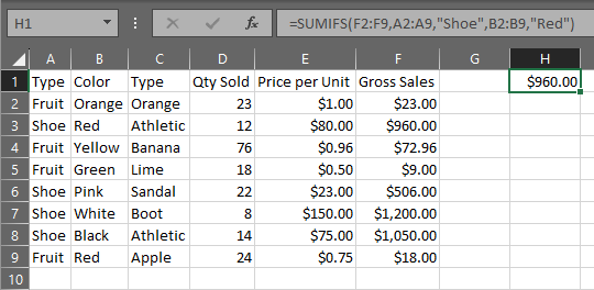
SUMIFS adds up numbers in a range based on multiple criteria. If you need to find the total sales for a specific product in a specific region, SUMIFS has it covered, whether you want the total sales for all red shoes or all red shoes sold in Colorado.

Example: “=SUMIFS(F2:F9, A2:A9, “Shoe”, B2:B9, “Red”)” adds up the numbers in F2:F9, but only where A2:A9 is “Shoe” and B2:B9 is “Red”.

AVERAGE()

Syntax: AVERAGE(number1, [number2], …)

How I remember it: Average(of everything in this range) or Average(of these specific values)

AVERAGE, as the name suggests, calculates the average of a group of numbers. It’s perfect for finding the mean score on a test, or the average daily sales.

Example: “=AVERAGE(B2:B100)” calculates the average of the numbers from cells B2 to B100.

The picky one: AVERAGEIFS()

Syntax: AVERAGEIFS(average_range, criteria_range1, criteria1, [criteria_range2, criteria2], …)

How I remember it: Averageifs(values in this range, where the matching value in this other range, equals this)

AVERAGEIFS calculates the average of numbers in a range that meet multiple criteria. It’s perfect for when you need to calculate the average sales of a specific product during a specific time period.

Example: “=AVERAGEIFS(C2:C100, A2:A100, “ProductA”, B2:B100, “January”)” calculates the average of the numbers in C2:C100, but only for rows where A2:A100 is “ProductA” and B2:B100 is “January”.

MAX() and MIN()

Syntax: MAX(number1, [number2], …) and MIN(number1, [number2], …)

How I remember it: Max(among everything in this range) or Min(among these specific values)

MAX and MIN help you find the highest and lowest values in a set, respectively. Whether you need to know the highest score on a test, or the lowest sales day of the month, these functions are a breeze to use.

Examples: “=MAX(C1:C50)” returns the highest value from cells C1 to C50. “=MIN(C1:C50)” does the opposite, finding the lowest value.

The picky ones: MAXIFS() and MINIFS()

Syntax: MAXIFS(max_range, criteria_range1, criteria1, [criteria_range2, criteria2], …) and MINIFS(min_range, criteria_range1, criteria1, [criteria_range2, criteria2], …)

How I remember it: Maxifs(everything in this range, where the matching cell in this other range, equals this)

These two functions find the maximum and minimum values in a range, but with a twist. They only consider values that meet one or more criteria. For instance, if you want to find the highest sales from a particular region, MAXIFS is your go-to.

Examples: “=MAXIFS(B2:B100, A2:A100, “East”)” finds the highest value in B2:B100, but only for rows where the corresponding value in A2:A100 is “East”. MINIFS does the same but finds the lowest value instead.

COUNT() and COUNTA()

Syntax: COUNT(value1, [value2], …) and COUNTA(value1, [value2], …)

How I remember it: Count(of cells in this range)

COUNT gives you the number of cells in a range that contain numbers. COUNTA is COUNT’s big brother. It counts the number of cells in a range that are not empty, regardless of whether they contain numbers, text, logical values, errors, or empty text (“”).

Examples: “=COUNT(D1:D100)” counts the cells with numbers from D1 to D100. “=COUNTA(D1:D100)” counts all cells that aren’t empty.

The picky one: COUNTIFS()

Syntax: COUNTIFS(criteria_range1, criteria1, [criteria_range2, criteria2], …)

How I remember it: countifs(values in this range, where the value in this other range, equals this)

COUNTIFS is a counting machine. It counts the number of cells in a range that meet multiple criteria. For example, you could use it to count how many sales were made by a specific salesperson in a specific month.

Example: “=COUNTIFS(A2:A100, “SalespersonA”, B2:B100, “February”)” counts the cells in A2:A100 that are “SalespersonA” and where the corresponding cell in B2:B100 is “February”.

ROUND(), ROUNDUP(), and ROUNDDOWN()

Syntax: ROUND(number, num_digits), ROUNDUP(number, num_digits), ROUNDDOWN(number, num_digits)

How I remember it: round(this value, to the nearest # digits after the decimal)

These three functions let you control how you round numbers. ROUND uses standard rounding rules, ROUNDUP always rounds up, and ROUNDDOWN always rounds down. You specify the number of decimal places with the num_digits argument.

Examples: “=ROUND(E5, 2)” rounds the number in cell E5 to two decimal places. “=ROUNDUP(E5, 0)” rounds the number in E5 up to the nearest whole number.

As a side note, it’s important to remember that all of these conditional (picky) versions have a most common usage where you’re matching a specific value, but the actual logic behind them can be carried far beyond that. Instead of saying “only for red shoes”, you can do other Boolean (true/false) logic in them as well. So you can add all banana purchases where the purchased quantity was 1, or where the purchased quantity was >50 (who does that?).

In short, if you can do it in an if formula, you can do it in a conditional math formula. Both work on the principle of Boolean logic tests, and use some evaluation that equates to a true or false to determine the outcome, so feel free to experiment.

Still me. Yep. Same dude.