Recommended Song for this breezy project:

Buckle up, data enthusiasts! Today, we’re going on a whirlwind adventure. We’re stepping away from the safe haven of our data centers and stepping right into… the heart of a tornado!

Oh, no need to look so terrified – we’re not really going to put you in the path of a twister. Instead, we’re going to let you sit comfortably at your desk and bring the tornadoes to you! That’s right, folks! We’re diving into the exciting world of automated data acquisition, and our data du jour is tornado data from the National Oceanic and Atmospheric Administration (NOAA).

So, are you ready to take your Excel skills up a notch? Are you excited to see how you can extract, merge, and clean data from the web, all while sipping your morning coffee? Most importantly, are you eager to see how we can turn raw, disjointed data into a visual feast in the form of a 3D map, showing the hot zones for tornadoes?

If the answer is a resounding yes, then roll up your sleeves, and let’s get started! There’s a tornado of knowledge coming your way, and it’s about to sweep you off your feet!

Project ‘Whirlwind’ commencing in 5… 4…

1) Start your engines! We’re about to embark on a digital scavenger hunt for our data sources. Be it in a folder tucked away in your PC, lurking on a network drive, or even across the big wide web, your data can spring up from anywhere. For this tornado of a task, I’ve sourced my data from the following links:

Source: Storm Prediction Center Maps, Graphics, and Data Page (noaa.gov)

• 2022: https://www.spc.noaa.gov/wcm/data/2022_torn.csv
• 2021: https://www.spc.noaa.gov/wcm/data/2021_torn.csv
• 2020: https://www.spc.noaa.gov/wcm/data/2020_torn.csv

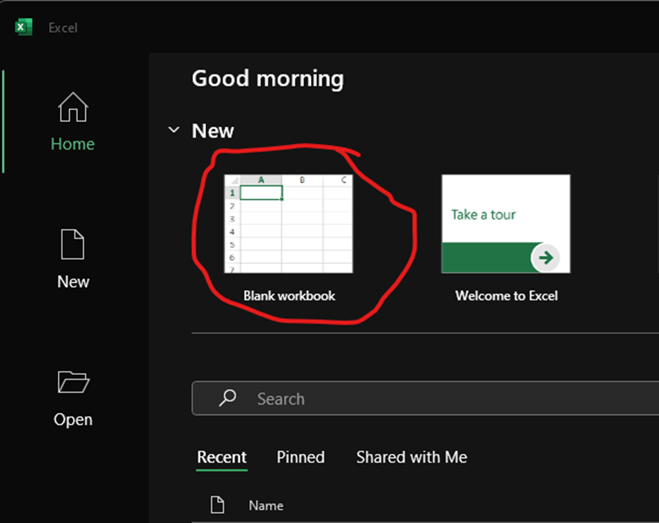
2) Let’s power up Excel and start with a fresh, clean slate – a brand new blank workbook right from the home screen.

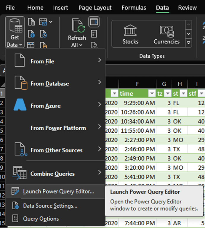
3) My tornado data comes in CSV format. I’ll dive into the ‘Data’ tab and select ‘Get Data’, followed by ‘From File’, and finally ‘From Text/CSV’.

4) Now, Excel wants to know if we’re friends, or rather, if we’re authenticated. Usually, it might ask for your organization’s credentials, but for this whirlwind journey, we can select ‘anonymous’, since this is a public dataset available to anyone. We’ll bypass our usual ‘Transform Data’ step and load all three data sources by repeating the same steps.

Step 5) It’s time to open up the Power Query Editor from the ‘Data’ menu.

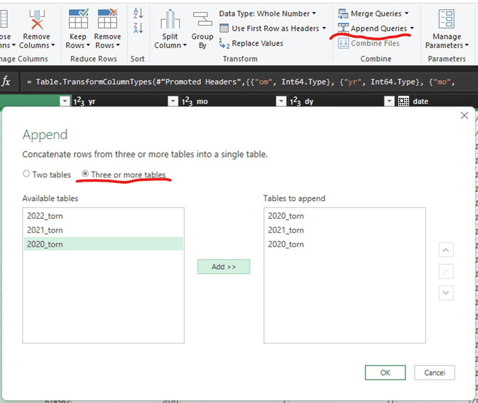
6) In the ribbon above, let’s select ‘Append Queries’. We’re about to mash all our source tables into a brand new one, so be sure to choose the ‘Append as new’ option, and make sure you click the bubble to indicate we’re combining three or more tables.

7) Let’s christen our new table with a name that actually makes sense – how about “NOAA Tornadoes”? We’ll do this by double-clicking on the table name and typing the new one in. Also, it’s time to do some spring cleaning by reviewing the column names and data types that Excel assigned on import to ensure they’re in tip-top shape.

• If you get a privacy notification, you can choose the option to ignore privacy for this file. You may want to review it for more sensitive information, but this is a publicly available dataset.
• It’s always helpful to find documentation for column names if you’re not sure what the dataset’s abbreviations mean. In this case, we can look them up here: https://www.spc.noaa.gov/wcm/data/SPC_severe_database_description.pdf

8) We’ll be trimming some excess fat by removing the FIPS codes (unless you’re keen to know which county has the most twisters). After that, we’ll tidy up the data types a bit – the loss estimates will get a currency makeover after we rename the columns.

9) All set? Great! Now hit the ‘Close and Load’ button on the left side of the home tab.

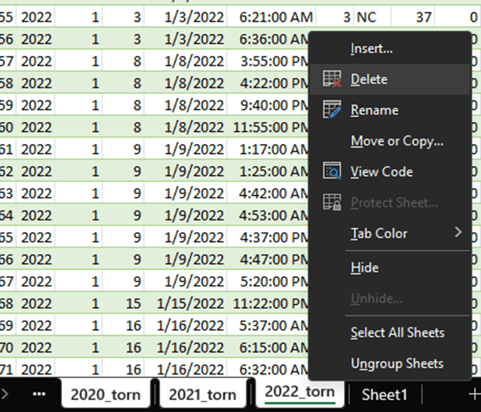
10) Voila! Excel has prepared a new worksheet named after your query. This will be our base camp moving forward. So let’s take a quick detour to delete the original three data source sheets and any other unnecessary sheets (looking at you, Sheet1!).

11) Now, for some magic! Head over to the ‘Insert’ tab on the ribbon and choose ‘3D Map’. If this is your first time, Excel might ask for permission to enable the add-in. Go ahead and grant it – the result will be worth it!

12) Now let’s put our data to work. Just like a pivot table, we’ll arrange our data fields. We’ll use a heat map visualization for this project with the starting latitude and longitude for positioning. Oh, and let’s bump up the radius of influence value to around 260% to cover our bases.

13) Our heat map highlights tornado hot spots, but we want more – we need details on damage and severity. Let’s add another layer that includes injury indicators, and use the bars this time, so that it acts similar to a pin. Feel free to play around with the color options (I’ve gone with bright orange for visibility).

14) If we go to both layers, and pop the date field into the time box… hit the play button at the bottom of our map visual. Watch as your data springs to life, showing the progression and build-up of tornado events over time. Truly a sight to behold!

15) Here’s where your creativity can run wild! You can experiment with other data points – the 3D maps tool is a free, versatile instrument for geographically visualizing your data. Once you’re satisfied, let’s bid goodbye to the 3D Maps (just close the window) and return to our trusty Excel workbook.

16) And just like that, we’re halfway through our data rollercoaster! We’ve:

• Found a treasure trove of data online.
• Imported that data into Excel in multiple chunks.
• Fused those chunks into a new, shiny query, and given the resulting table a makeover.
• Imported that table into our workbook and took a scenic tour with Excel’s underappreciated 3D Maps tool.

17) But what if you want this process to happen regularly, without manual effort? Worry not, we’re about to automate this task!

18) Back in our Excel Workbook, hit Alt+F11 on your keyboard (or open the Visual Basic Editor from the Developer tab on your ribbon).

19) After the editor opens, double-click on ‘ThisWorkbook’ in the Project pane and type in the following magic spell (code):

Private Sub Workbook_Open()
    ActiveWorkbook.RefreshAll
    ActiveWorkbook.Save
End Sub

20) This code we’ve typed in is quite the Excel whisperer – it tells Excel to run the code whenever the workbook is opened (as long as your security settings allow it). This nifty bit of VBA just refreshes the queries (keeping our data fresh as a daisy) and then saves the workbook with those updates. Isn’t that cool?

21) Close your VB Editor and save your workbook as a Macro-Enabled Workbook.

22) But why stop there? Let’s make this even easier by ensuring we don’t even have to open the file to update the data! For that, we’ll need a simple VBScript and the Task Scheduler.

23) VBScripts use the same language as VBA, but in this case, we just need it to open the workbook, run the macro, wait for a while to let the updates sync, and then close the workbook. It’s as simple as it gets!

24) Now, whip out your notepad (from the start menu) and insert the following text, replacing “\path\to\your\Workbook.xlsm” with the actual path to your NOAA Tornadoes workbook. Then, save this file as “NOAATornadoes.vbs” in your project folder.

Dim xl
Dim xlBook
set xl = createobject("Excel.Application")
xl.Application.Visible = True
xl.DisplayAlerts = False
Set xlBook = xl.Workbooks.Open("\\path\to\your\Workbook.xlsm", 0, False)
WScript.Sleep 10000 'Sleeps for 10 seconds
xlBook.save
xl.ActiveWindow.close True
xl.Quit

26) Double-click your script to run it. If all goes well, you’ll see Excel open, do some work for about 10-12 seconds, and then close again.

• If it gets blocked, you’ll likely need to change your macro and external data connection settings in the trust center to allow the query and macro to work.
• You can get there in Excel by going to File->Options->Trust Center->Macro Settings (or External Content). Some caution is advised here, since you’re technically allowing ANY macro to run, and ANY data source to be queried from excel on the computer you make these changes to. Never open a macro enabled file you don’t trust or haven’t already verified with macros disabled.

27) Now that we’ve automated opening our workbook and updating it, let’s make it even more effortless by having it run without our intervention using the Task Scheduler.

28) Open the Task Scheduler (you can simply search for it in your Start Menu).

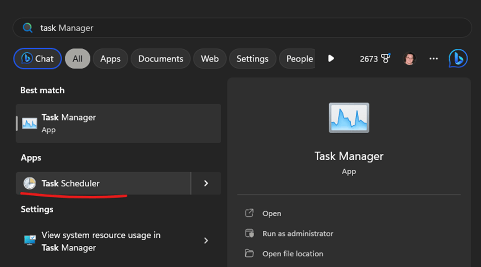
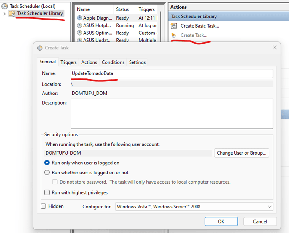
29) Once it opens, click on “Task Scheduler Library,” then find and click the “Create Task” button in the Actions pane.

30) You’ll be presented with a “Create Task” Window. Begin by assigning your task a unique and identifiable name.

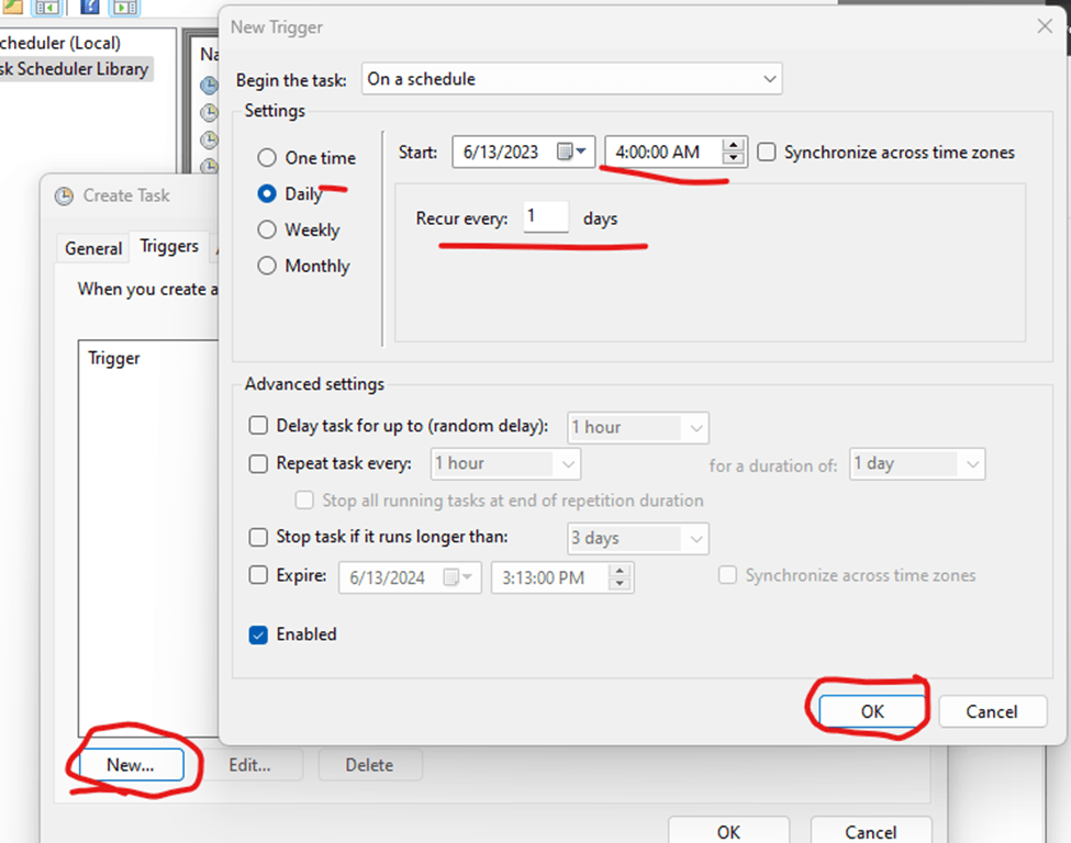
31) Next, we move on to Triggers. Click “New”, set up your schedule for this report to refresh. I’m opting for a daily, early morning refresh, but feel free to customize it to your liking. Don’t forget to hit “OK” when you’re done.

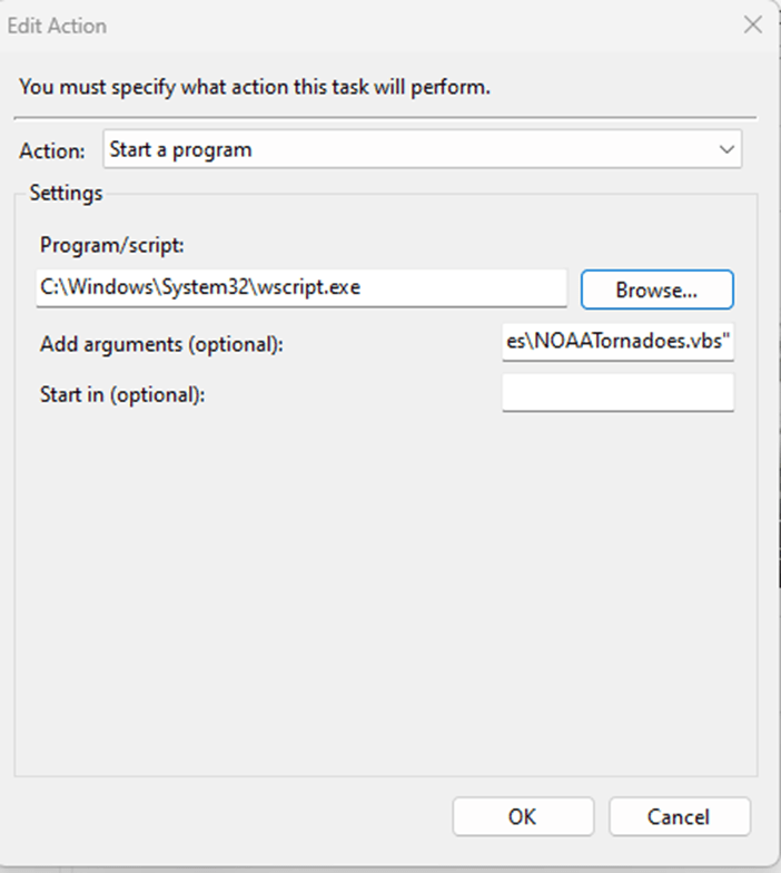
32) It’s action time! Navigate to the Actions tab, click ‘New,’ and browse to locate the script we created earlier on your local PC. After you’re done, click “OK”.

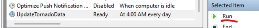
33) And with that, we’re almost home! Click “OK” one last time on the Create Task window, and voila! Your new scheduled task will now be listed in the Task Scheduler Library List! To test it, select it from the list and click the “Run” button in the actions pane.

• Side note, if it doesn’t run, remember that computers can be picky. In my case, when I tried to run it, it didn’t like that the script was saved in OneDrive, and that stopped it from launching. With a few minutes of googling, we end up fixing that by double clicking our task, and changing the action we set up earlier to this configuration, after which, it worked like a charm:

34) Bravo! You have now established a fully automated data acquisition process using nothing more than Excel, the internet, and built-in Windows resources! Now, your data updates will be as fresh as a morning’s dew, and you didn’t even have to lift a finger!

Wrapping Up Our Twister Tour: We’ve Caught the Tornado, Now What?

Well, there you have it, data storm chasers! We’ve navigated the tornado alley of automated data acquisition, and emerged triumphant, not a hair out of place. With a few simple steps, some handy Excel magic, and a splash of VBScript, we’ve tamed the tempestuous twisters into a manageable dataset, all from the cozy comfort of our desks.

We’ve ventured on this wild data journey together, wrangled tornado data from the internet, tamed it into submission, and ended up with a pretty stellar 3D Map along the way. We’ve even set up an automated task to keep our data fresh as a spring morning after a tornado… Wait, is that too soon?

Jokes aside, this journey has shown us the strength of Excel and VBScript. We have created something pretty amazing out of raw, publicly available data. More importantly, we’ve automated the entire process, saving us precious time for more fun data endeavors. Don’t worry, the way we’ve set things up, the workbook can be opened manually without closing itself every time (remember, the macro is just to refresh and save. The VBScript is how we close the workbook when it runs as a scheduled task), so you can still enjoy that map while the task scheduler and VBScript keep the data up to date for other tools and systems that may use it!

Remember, in the world of data, every day is a new opportunity for adventure. So, let’s continue to chase those data storms and unearth the treasures that they hide. Until our next data expedition, stay curious, stay adventurous, and most importantly, stay safe – there’s no need to chase actual tornadoes when we can bring them right to our Excel sheets!