Hola, data enthusiasts! Ready to venture deeper into the world of Excel lookup and logic functions, and take a look at why they’re some of the most commonly used tools in the business? We’re taking a journey today through the landscape of Logical and Lookup functions. While logical functions allow us to have some control over the process of how our data is transformed, lookup functions allow us to pull in more context from other sources and enrich our datasets with new information. With one adding context and clarity, and the other helping with classification and flow control, we can think of them as our friendly guides in making decisions and navigating through your data.

We’ll start with the lookups, since they’re a more common need with beginner and intermediate users, and I’ll note in advance that there are other options available in the tools, but some of them are only available with specific add-ins, or in some of the newest versions of the software. Vlookup, Hlookup, and Index/Match, on the other hand, are basically the uncontested champions when it comes to lookups in Excel.

VLOOKUP() – The Data Detective

Syntax: VLOOKUP(lookup_value, table_array, col_index_num, [range_lookup])

How I remember it: VLOOKUP(find this thing, in this table, and give me the data from this column)

VLOOKUP is your private detective, tirelessly combing through rows of data to find what you’re looking for.

Example: =VLOOKUP("ProductA", A2:C100, 3, FALSE) searches for “ProductA” in column A and returns the corresponding value from column C.

HLOOKUP() – The Horizontal Scout

Syntax: HLOOKUP(lookup_value, table_array, row_index_num, [range_lookup])

How I remember it: HLOOKUP(find this thing, in this table, and give me the data from this row)

HLOOKUP() is the horizontal counterpart to VLOOKUP(). If your data is arranged horizontally, this is the function you need.

Example: =HLOOKUP("January", A1:M3, 3, FALSE) searches for “January” in row 1 and returns the corresponding value from row 3.

INDEX() and MATCH() – The Dynamic Duo

Syntax: INDEX(array, row_num, [column_num]), MATCH(lookup_value, lookup_array, [match_type])

How I remember them: INDEX(in this range, find the cell at this row and column), MATCH(find this thing, in this list)

INDEX() returns the value of a cell in a specified position in a range, while MATCH() returns the position of a lookup value in a row, column, or table. Used together, they’re a powerful combo that can replace VLOOKUP or HLOOKUP.

Example: =INDEX(C2:C10, MATCH("ProductA", A2:A10, 0)). Here, MATCH() finds the row number of “ProductA” in the range A2:A10, and then INDEX() uses that row number to return the value from the same row in the range C2:C10.

That pretty much covers what you’ll need in the majority of cases where you want to attach data from one source to another, but as I mentioned at the top, there are other options out there that could be worth exploring and that you may like more for your common usage. The options and use cases are nearly endless, but I highly recommend learning at least one solid lookup function for both vertical and horizontal lookups (hint: Index(Match()) can do both. And lookup values in any direction.), and practicing them until you’re comfortable.

In one of our recent articles, we covered the idea of unique keys, and how they can be leveraged to link information between tables via relationships or lookups like the ones we’ve discussed here; most often you’ll be using lookups to pull additional information from another table or range to add information to one of those keys. As a practical example, you may lookup a product’s Description, height, length, width, and weight based on the item number, or pull in a customer’s address based on their account number.

Now, on to the logic, when you want to categorize things, or do different things with the information based on the conditions or values of the data itself. Perhaps you want to classify customers into groups based on annual spend to pre-define the buckets for a histogram? Logical functions like If and Switch can help you do that, and functions like And, Or, and Not can help you fine tune how they’re applied.

IF() – The Decision Maker

Syntax: IF(logical_test, value_if_true, value_if_false)

How I remember it: IF(this is true, then do this, otherwise do this)

IF() is your personal decision maker in Excel. It’s like a tiny robot that takes a condition, checks if it’s true or false, and gives you a result based on that.

Example: =IF(A2>10, "Yes", "No"). This formula checks if the value in cell A2 is greater than 10. If it is, it returns “Yes”, and if not, it returns “No”. It’s great for classifying data based on conditions.

Note: The IF function could be paired with other functions like AND, OR, NOT to create more complex decision-making formulas. Speaking of which…

AND(), OR(), NOT() – The Boolean Logic Trio

Syntax: AND(logical1, [logical2], …), OR(logical1, [logical2], …), NOT(logical)

How I remember them: AND(all of these things are true), OR(any of these things are true), NOT(this thing is true)

The AND, OR, and NOT functions in Excel are the building blocks of logic. AND returns TRUE if all conditions are true, OR returns TRUE if any condition is true, and NOT returns the reverse of a given logical value.

Example: =AND(A2>10, B2<5) checks if the value in cell A2 is greater than 10 AND the value in B2 is less than 5. If both are true, it returns TRUE, if not, FALSE.

SWITCH() – The Multitasker

Syntax: SWITCH(expression, value1, result1, [default or value2, result2]…])

How I remember it: SWITCH(if this cell is, this value then do this, or this value then do this, or if not any of these then do this)

SWITCH() evaluates one value (the expression) against a list of values, and returns the result corresponding to the first matching value. If there is no match, an optional default value can be returned.

Example: =SWITCH(A2, "Red", "Stop", "Green", "Go", "Yellow", "Slow Down", "Invalid Color"). This formula checks the value in A2, if it’s “Red” it returns “Stop”, if “Green” it returns “Go”, if “Yellow” it returns “Slow Down”, and if it’s any other color, it returns “Invalid Color”.

Nested IFs vs. SWITCH – The Great Debate

Fair warning, I’ve seen this debate get rather heated at times, so I’ll say the views and opinions expressed here are my own, and not intended to try and convince you that one or the other is better. I’d honestly rather everyone learn to use both, as long as they keep a few best practices in mind when applying them.

If you’ve got a few conditions to test, you might find yourself wondering: should I nest a bunch of IFs, or should I go for SWITCH? Both can handle multiple conditions, but they do so in different ways. Let’s weigh up the best practices for each.

Nested IFs – The Classic Path

Nested IFs are often the first choice simply because we’re more familiar with them. They’re great for sequential conditions that need to be evaluated in a particular order, or when there’s a hierarchy to your data. IF statements also work well when you’re working with ranges of numbers or dates.

Example: =IF(A2<10, "Low", IF(A2<20, "Medium", "High")) labels a number as “Low”, “Medium”, or “High”. The conditions are checked sequentially, so order matters.

Essentially, it works like an old school coin sorter, where a given value may fit into several slots in the machine, but it’s going to go into the first one that fits. Here’s a comically simple (and tragically misused) SmartArt example that should help to visualize how nested ifs work, moving from left to right.

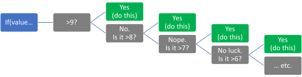
As long as you plan for how the logic will be applied, you can use this approach to get the result you want pretty much every time. However, when you have many conditions, nested IFs can become complex and hard to read. Excel also limits you to 64 nested IFs – but if you’re getting anywhere close to that number, it’s a sign you might need a different approach anyway!

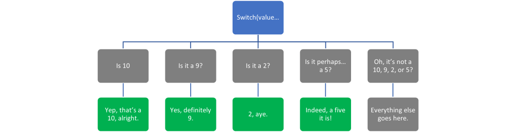
SWITCH – The Order-Agnostic Alternative

SWITCH, on the other hand, is order-agnostic. It’s perfect for when you’re dealing with a list of independent values or conditions. If your conditions don’t have a particular sequence, and you just need to check if your value matches one of the listed possibilities, then SWITCH is a great choice. It’s generally easier to read than a lot of nested IFs, too!

Example: =SWITCH(A2, "Red", 1, "Blue", 2, "Green", 3, "Invalid") assigns a number to a color. The conditions are checked independently, not in sequence.

However, SWITCH isn’t as flexible as IF. It can’t handle ranges or inequalities – it’s strictly about exact matching. If you need a catch-all ‘else’ condition, SWITCH provides for this with a default result at the end. As you can see below, the switch prefers exact category definitions, but can be used with logic tests if absolutely necessary (i.e. Switch(A2, And(A2>0,A2<10), “Value between 1 and 9”,…).

In Excel specifically, If you’re going to use a switch for more than a few conditions, I’d recommend using the Alt+Enter shortcut to format your formula so that each condition and outcome is on a separate line. I’ll still work the same way, but the line breaks will make it easier to read if you have to come back to it.

In conclusion, the choice between nested IFs and SWITCH comes down to your specific conditions and the order they need to be evaluated in. IFs are best for sequences or hierarchies, while SWITCH excels at handling lists of independent values. So, consider the nature of your data, the complexity of your logic, and the readability of your formula before choosing your path. Happy analyzing!

And now, let’s wrap things up…

Throughout this post, we’ve taken a deep dive into the world of Excel’s lookup and logical functions, exploring the vast potentials they bring to your data manipulation endeavors. These powerful tools open up a world of possibilities that stretch far beyond simple calculations.

We journeyed to the crossroads of HLOOKUP and VLOOKUP, exploring how these functions search for information in your data table. You learned how they look for a value in a specified row or column, and then return a corresponding value from a different row or column. And let’s not forget the dynamic duo of INDEX and MATCH. You’ve now heard about the magic of their combined power in finding specific data in your worksheet. These two combined can overcome the limitations of VLOOKUP and HLOOKUP, offering more flexibility in retrieving data.

We then moved on to logic, starting with the trusty IF function, a stalwart partner in any Excel user’s journey. You learned how this function can test a condition and return different results based on whether that condition is true or false. It’s the bedrock of decision-making within your worksheets, giving them the power to ‘think’ and ‘decide’.

Then we flipped the tables with the SWITCH function, introducing a different approach to handling multiple conditions. We discovered how SWITCH can be a neat, readable solution when dealing with a list of independent values that aren’t bound by a hierarchy or sequence.

Next, we posed a great debate: when to use Nested IFs and when to call upon SWITCH? We discovered that it’s not about which one is better, but rather which one is more suitable for the task at hand (This has been my opinion for years, and no one on Stack Overflow has convinced me otherwise). Both Nested IFs and SWITCH have their unique strengths that make them perfect for different scenarios.

Learning how these functions work and when to use each one can significantly streamline your data analysis process. And remember, the more you use these functions, the more familiar you’ll become with their nuances and potential, becoming an Excel power user in no time!